This manual describes the Force Sensor hardware and the locally written software that interfaces to it.
Hardware
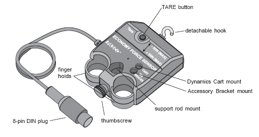
Our detectors are the Economy Force Sensor (Pasco CI-6746). It contains a strain gauge which generates a voltage when a force is applied to the receptacle that in the figure has the detachable hook screwed into it. The voltage is output to the 8-pin DIN plug which is typically connected to the U of T Data Acquisition Device, which in turn is connected to a PC running LabVIEW. The voltage that is generated ranges between -8 volts and +8 volts for forces between -50 N and +50 N.
The manufacturer quotes a sensitivity of 0.03 N, which we usually take to be the uncertainty in the measured force.
\(\Delta F = 0.3\ N\) (1)
 The voltage generated by the sensor tends to drift. Periodically be sure to have zero force applied to the sensor and press the TARE button.
Software
In research laboratories the standard software for data acquisition and process control is LabVIEW from National Instruments. The software for the Force Sensor was locally developed using LabVIEW. Such programs are called virtual instruments or more usually just vi’s.
We have developed three different vi’s for the Force Sensors:
- ForceSensor. This version is for a single force sensor plugged into Analog Sensor A on the U of T Data Acquisition Device.
- ForceSensors2. This allows two separate force sensors to be used. One is plugged into Analog Sensor A and the other into Analog Sensor B on the U of T Data Acquisition Device.
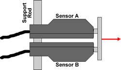 ForceSensorsDoubled. Sometimes we need to measure a force greater than the 50 N maximum that the Force Sensor is capable of measuring. When two force sensors are connected in parallel as shown, this vi reads the sum of the readings of the two sensors. One sensor should be plugged into Analog Sensor A and the other into Analog Sensor B on the U of T Data Acquisition Device.
Here we concentrate on the ForceSensor vi. ForceSensors2 offers only a subset of the full functionality of ForceSensor; some brief remarks about this vi appears at the end of this document. ForceSensorsDoubled has the same functionality as ForceSensor.
All three vi’s sample the force 100 times a second.
Here is a screen shot of he Force Sensor vi.
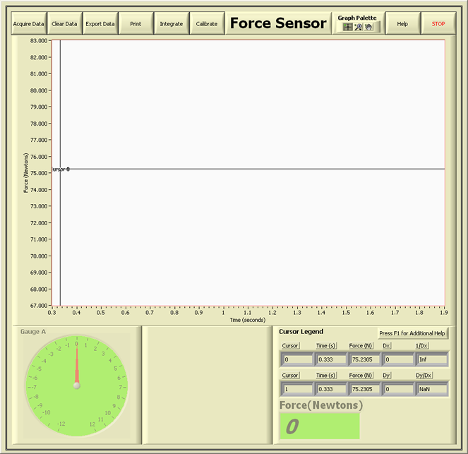
Along the top left part of the front panel are a row of buttons. From left to right they are:
- Acquire Data. Click to begin collecting data: the button will turn green. Click again to stop collecting data.
- Clear Data. Only active when you are not collecting data, this clears all previously collected data and removes it from memory.
- Export Data. Only active when you are not collecting data, this exports the data as time-force pairs to a file. You will be able to choose any title that you wish for the dataset. Below we discuss various ways of changing the view of the data in the force-distance plot: these do not affect the data saved by the Export Data function, will always saves all the data currently in memory.
- Print. Only active when you are not collecting data, this prints the front panel to the default printer.
- Integrate. Only active when you are not collecting data, this calculates the area under the force-time curve. Further details on this are given below.
- Calibrate. Only active when you are not collecting data, this allows you to suspend a known mass from the force sensor to calibrate its readings. When the ForceSensor program first starts, the default calibration value is used. When you click on the Calibrate button, in the dialog box that appears choosing ‘Yes’ will allow you to calibrate the sensor; choosing ‘No’ will use the current calibration setting; choosing ‘Cancel’ causes the program to revert to the default calibration value it had when it first started.
Along the top right of the front panel are three buttons:
- Graph Palette. We will describe this below in the Working With Graphs and Cursors section.
- Help. By hovering the mouse over the front panel, a brief description of each component of the panel will appear. This Help button will cause a more complete description of the component to appear in a separate window. Further information on the program will appear in the default browser by pressing F1. The most complete description of the software is the document you are now reading.
- STOP. Click to exit the program.
The central area of the front panel is a plot of the force versus time. Further information on working with the graph appears below in the Working With Graphs and Cursors section. At that time we will also discuss the Cursor Legend area in the lower right of the front panel.
The lower left part of the window is a gauge showing the current value of the force. This value is also displayed numerically in the lower right part of the window.
Working With Graphs and Cursors
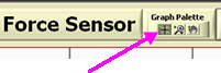 When the program starts, there are two cursors, called Cursor 0 and Cursor 1, located to the left of the force-time plot. Towards the upper right part of the front panel is a Graph Palette control. There are three possible functions, and the left-most one allows you to move the cursors by dragging them with the mouse. The selected function is gray. The figure to the right shows the palette when it is set so you may move the cursors with the mouse.
The middle function of the Graph Palette is the zoom tool, and the right one allows you to move the plot with the mouse.
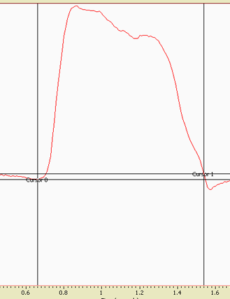
Here is part of a force-time plot with the cursors selecting a region of the data.
Each cursor consists of a vertical and a horizontal line which intersect on the data curve.
The time and force values appear in the Cursor Legend panel just below the graph. Also shown are the difference in times between the two cursors, labeled Dx, and the difference in the forces, labeled Dy. The values of 1/Dx and Dy/Dx are also shown.
By default, the scale of the axes of the plot shows all the data. You may change the scale of an axis by choosing a value on the far left or far right of the axis label, double clicking it, typing in the new value and pressing Enter.
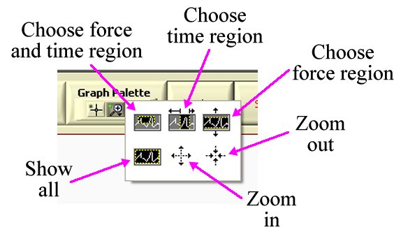
If you click on the zoom tool, the middle of the three buttons in the graph palette, a drop-down menu appears as shown to the right. The two most used of the items in the menu are:
- Choose time region: you may “paint” in a horizontal time region with the mouse, and the plot will zoom in on the selected region.
- Show all: displays the entire data plot. This undoes any other selections you have made with the zoom tool.
The other functions are:
- Choose force and time region: paint in a rectangular area of force and time values to zoom in on that region.
- Choose force region: paint in a vertical force region with the mouse to zoom in on that range of forces.
- Zoom in and Zoom out: Zoom in and out of the plot with the mouse.
The Area Under the Curve
The Integrate button on the front panel calculates the area under the force-time plot between the two cursors. The result is displayed in the area at the bottom and in the centre of the front panel.
The integrate function is fairly simple. Assume we have N time-force pairs:
\(({t_1},{F_1})\,\,({t_2},{F_2})\,...\,\,({t_N},{F_N}) \)
Then the area under the curve is calculated as
\(\sum\nolimits_{i = 1}^{N - 1} {\frac{{\left( {{F_i} + {F_{i + 1}}} \right)}}{2}\,\left( {{t_{i + 1}} - {t_i}} \right)} \) (2)
However, there is a subtly to the calculation. Say we have data that looks like the following figure.
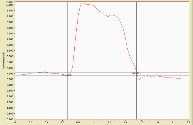
There appears to be a background force of about 4 N, and between 0.66 and 1.54 seconds there is a pulse. Typically we wish to subtract the background from the pulse. Thus the values of the force used to calculate the area has the value for Cursor 0 subtracted from them. Thus the calculated area under the curve is for the region between the cursors and above the horizontal line of Cursor 0.
The ForceSensors2 vi
This vi has two gauges and numerical readouts for the forces. The labels on the gauges and readouts correspond to the Analog Input channel on the U of T Data Acquisition Device to which the sensor are connected.
You may find it helpful to know that:
- In the plot, the red curve is for the sensor connected to Analog Input A, and the blue curve is for the sensor connected to Analog Input B.
- Cursor 0 tracks the time-force data A; Cursor 1 tracks the time-force data B.
This manual was written by David M. Harrison, Dept. of Physics, Univ. of Toronto in October 2008.
The figure of the sensor is from the Pasco manual 012-06909b.