This manual describes the Motion Sensor hardware and the locally written software that interfaces to it.
Hardware
Our detectors are the Motion Sensor II (Pasco CI-6742). Calling this device a Motion Sensor is a bit misleading: it measures the distance of an object from the detector, not the motion of the object. The device was originally invented by the Polaroid Corporation as a range finder for cameras.
Principle of Operation
Behind the brass screen is a transducer that generates an ultrasonic sound pulse. The same transducer generates a signal when the echo of the pulse is received. By measuring the time \(\Delta t\) between the generation of the pulse and receiving the echo, if the speed of sound is v then the distance d between the sensor and the object is:
\(d =\frac{v \Delta t}{2}\)
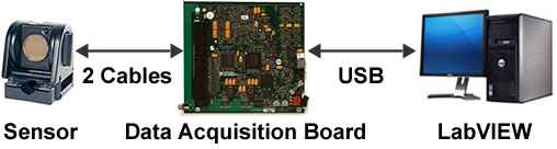
The sensor is connected to a Data Acquisition Board (DAQ), which then connects via a USB cable to a computer. A program on the computer, written in LabVIEW, controls the sensor and reads the distance through the DAQ. The DAQ is housed in a locally designed and fabricated Data Acquisition Device.
 The sensor can not measure distances less than 15 cm. The maximum distance it can measure is about 8 m.
The Sensor
 The figure shows some details of the sensor. We will go though those details
Narrow/Std Switch
This controls the width of the ultrasonic sound wave. The Std setting is a wide beam, and the Narrow setting restricts the sound wave to about 15 degrees. On some sensors instead of being labeled Std and Narrow the switch has two icons: one is of a cart (the narrow position) and the other is of a person (the Std setting).
Typically this will be set to the Narrow position. This reduces the chance of the sensor registering a false target, and also reduces the sensitivity to noise.
For poorly reflecting targets, you may need to set the switch to Std.
Target Indicator LED
This flashes when the sensor has acquired a target.
Positioning Dial
This allows the orientation of the sensor to be rotated.
Note: when operating in Std mode (a wide sound wave), you may need to rotate the sensor so that the angle the sound wave makes with the horizontal is 5 or 10 degrees. This is to keep the wave from bouncing off a tabletop etc.
Phone Plugs
These are plugged into the corresponding terminals on the Data Acquisition Device. On the left side of the Device are two pairs of terminals labeled Digital Channels; each pair has one labeled with a yellow circle and the other with a black circle. The corresponding yellow and black plugs from the sensor are plugged into pair labeled 0, yellow to yellow and black to black.
Mounting on a Dynamics Track
Often you will wish to mount the sensor on a dynamics track. The figure shows how to do this.
Software
In research laboratories the standard software for data acquisition and process control is LabVIEW from National Instruments. The software for the Motion Sensor was locally developed using LabVIEW. Such programs are called virtual instruments or more usually just vi’s.
To start the software, double click on the Motion Sensor icon on the desktop.
It is an excellent idea of have a look at the various parts of the window that will open, to get a rough idea of what information and controls are available to you.
Here is a screen shot of the upper left part of the window:
The right-facing arrow, circled in the screen shot, starts the virtual instrument. There is a button labeled Quit (not shown) in the upper-right corner of the window which stops the instrument.
You may have already noticed that there are a number of tabs across the top of the vi. We will describe them.
Collect Tab
 This is the tab that gives controls to start and stop the sensor and collect data. Here is a screen shot of part of the contents of the tab:
The Start Detector button starts the sensor. When clicked the button will show a green light. You may be able to hear the sensor clicking. When the detector receives an echo the green LED on the front of the sensor will flash. Clicking on the Start Detector button again stops the detector; the green light on the button goes out.
To collect distance-time data, click on the Collect Data button. You may only do this after you have started the detector. Data collection will continue until you click on Collect Data again.
Sometimes the hardware/software does not set up communication with the sensor. In this case the green LED on the sensor will not flash.
- Stop the detector by clicking on the Start Detector button again.
- Unplug the sensor from the Data Acquisition Device and plug it back in.
- Re-start the detector by clicking on the Start Detector button.
When you are collecting data, the distance data is displayed in the graph which is not shown in the above figure.
When you stop collecting data, if you start collecting data again the old data is deleted.
Analyze Tab
After distance data has been collected, this tab slows you to do some analysis and trimming of the data. Here is a screen shot of the upper part of the tab:
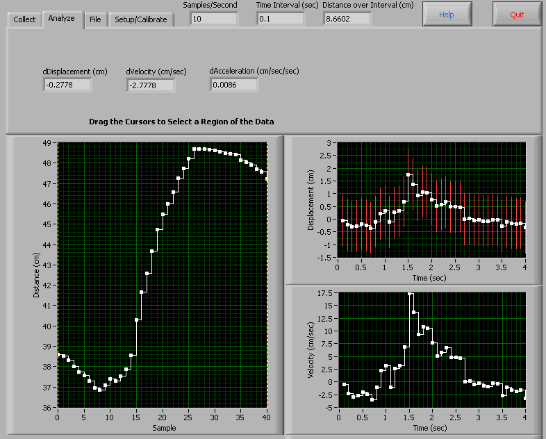
On the left is a graph of the distance data: this is the distance of the object from the sensor. This is the same data that you saw in the graph in the Collect tab. Note that the horizontal axis is the sample number.
On the upper right, the displacement data are shown, with the horizontal axis now being the time in seconds. Recall that if two successive distance measurements are ri and ri+1, then the displacement is ri+1 - ri.
Note that uncertainties in the values of the distance have been estimated and are displayed in the time-displacement plot. Details of how those errors have been estimated appear in the Appendix to this Guide. In a future release of the software you will be able to substitute for the values of the errors in the distance values.
Below the distance-time plot is a plot of velocity versus time, calculated from the displacement-time data. In a future release of the software, this plot will also have uncertainty bars.
Below the velocity-time plot and not shown is a plot of acceleration versus time, calculated from the velocity-time data. It too will have uncertainty bars soon.
In the raw distance-sample plot on the left of the Analyze tab there are two cursors, represented by vertical dashed yellow bars. Initially they are on the far left and right of the plot. You may grab these with the mouse to select only the data between them. These “trimmed” values are what are then used in the three graphs to the right of the window.
By default the scales of the graphs are set to show all of the data. Sometimes an extraneous datapoint means that this scaling is not what you wish. To change the scaling of any plot:
- Double click on the maximum or minimum value displayed on the axis whose scale you wish to change.
- Enter the new value and press Enter on the keyboard.
File Tab
This tab allows you to save the distance-time data, including errors in the distance, to a file. When you click on the Save button you will have the opportunity to change the default title of the dataset. If you “trimmed” the data in the Analyze tab it is that trimmed data that are saved.
Setup/Calibrate Tab
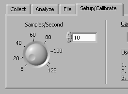 Here is a portion of the Setup/Calibrate tab:
You may adjust the number of samples per second being collected either:
- With the round knob, or
- Using the arrow keys, or
- Typing in the value that you wish in the text window.
By default, the software assumes the speed of sound is 344 m/s. This is usually a good value. However, you may calibrate the speed of sound by using the part of the tab that is not shown in the figure.
Appendix
Here we discuss how we arrived at the estimated uncertainties in the values of the measured distance. It assumes some knowledge of the standard deviation, which we only briefly review.
We repeat the measurement of some physical quantity x say N times. From the data we calculate an estimated mean of the values \(\bar{x}_{est}\). Then the spread in the values is expressed by the standard deviation estimated \(\sigma_{est}\), which is calculated from:
\({\sigma _{est}} = \sqrt {\frac{{\sum {{{({x_i} - {{\bar x}_{est}})}^2}} }}{{N - 1}}} \)
We can call the numerator of the expression inside the square root the sum of the squares of the residuals, i.e. the sum of the square of the difference between each individual data point and the estimated mean.
We can call the denominator of the expression inside the square root the number of degrees of freedom, which is just the number of data points minus that fact that we have used the data to calculate the estimated mean
It is reasonable to associate this estimated standard deviation with the uncertainty in each individual datapoint xi.
When we fit data to some polynomial, good fitters will tell us what the sum of the squares of the residual for the fit are. Just as for the standard deviation, this is the sum of the square of the difference between the value of the dependent variable of each data point and the value given by the fitter. Some fitters will also tell us the number of degrees of freedom of the fit: it is just the number of data points minus the number of terms in the polynomial to which we are fitting the data. Then the equivalent of a standard deviation for a fit is:
\(\sqrt {\frac{{sum\,of\,the\,squares}}{{degrees\,of\,freedon}}} \)
This can reasonably be taken to be the uncertainty in the values of the dependent variable.
We used the Motion Sensor hardware and software to collect some data for a cart on a track. We then used the PolynomialFit program to fit the data to the appropriate polynomial. Then from the sum of the squares of the residuals and the degrees of freedom of the fit we could calculate the estimated error, and code that value in the Motion Sensor vi.
This guide was written by David M. Harrison, Dept. of Physics, Univ. of Toronto in September 2008. Many of the figures in the Hardware section are cut and pasted from the Pasco Instruction Sheet 012-08624A
The Motion Sensor vi was written by David Rogerson, Dept. of Physics, Univ. of Toronto in the Summer/Fall of 2008 with input from David M. Harrison and Larry Avaramidis.