Kinematics

Activity 1

If you ignore friction, a cart rolling down a hill accelerates at \(a=g\sin\theta\). You are going to measure g by rolling a cart down a track.

Open Capstone and set up the motion sensor.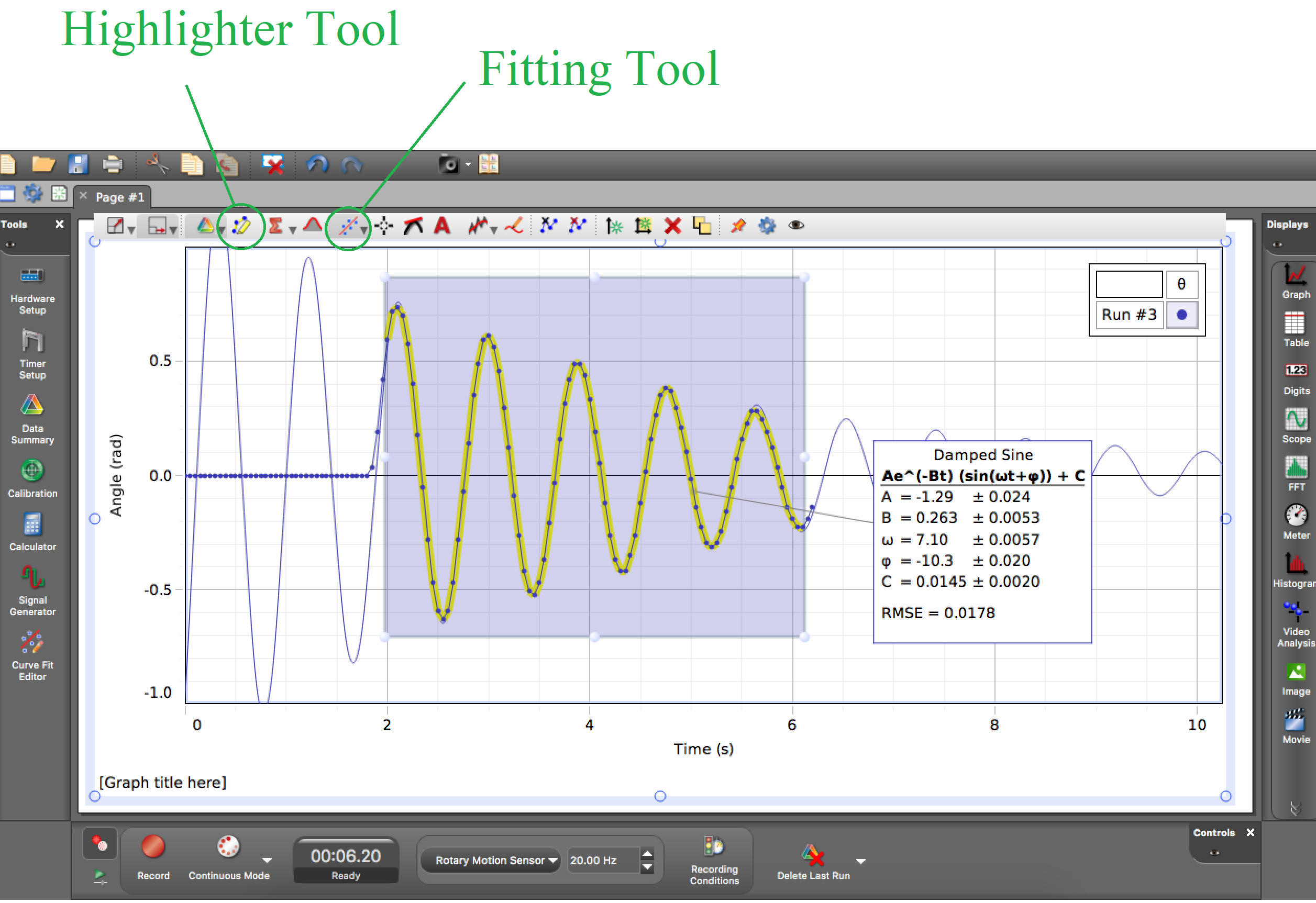

First make sure your track is level. Then use the metal bricks under one side of the track to raise it at an angle. Measure that angle as accurately as you can. For best results you probably want to use trigonometry and the vernier calipre. Take position-time data of the cart as it rolls down your hill. First: plot a(t) and find the average. Next: plot x(t) and fit the x(t) data to a parabola and use that value (actually it’s off by a factor of 2, you should know why). The image on the right shows how to fit your x(t) data by first highlighting the desired data and then using the fitting tool. The arrow on the fitting tool lets you select a function (you want a quadratic).

Estimate the uncertainties of both methods and discuss which is better. Note that when you fit the x(t) data using the software, it tells you the uncertainty of the fitting calculation (we’ll call it the fitting uncertainty), so you only need to estimate the uncertainty when using the a(t) graph.

What is your value of g, including uncertainties? Is it consistent with the accepted value of 9.8 m/s²? The best way to evaluate the consistency is to subtract 9.8 from your value and then compare that result with your uncertainty. If the difference is smaller than the uncertainty then they are experimentally equal. If the difference is up to 3 times larger than the uncertain then a physicist would not be comfortable claiming they were different and so would conclude that they are consistent.

Note: you calculated g from two measured quantities, both of which have uncertainties. In addition, your motion sensor has a measurement uncertainty. Since your calculation does not involve addition or subtraction, your uncertainty for g is the same percentage value as the largest percentage uncertainty of all three uncertainties.

Summary: you should have measured g and have a concrete way of comparing your value with the accepted value. Your result might "disagree" with the accepted value, but that's okay as the following activities will help us figure that out.

Activity 2

Now find g when the cart goes uphill instead of downhill. Don’t repeat all of step (2), just use the best method. Compare your results of uphill and downhill, including uncertainties. Are they consistent with each other? Is ignoring friction wise?

Summary: along with activity 1, you now have 2 different values of g, and should be able to explain any "disagreements" with the accepted value.

Activity 3

If we include friction, the cart should accelerate at \(a=g\sin\theta-\mu g \cos\theta\) if going downhill. Use the small angle approximation and it becomes \(a = g\theta -\mu g\). This is a straight line. Take data for several angles (by changing how many metal bricks you use), plot a(θ) and find the slope. NOTE: you must plot the angle in radians, not degrees! The small angle approximation only works in radians. 

Note: you can measure the angles most accurately with trigonometry and measuring the slope length (hypotenuse) and height (opposite side). The hypotenuse is the distance along the track between the two legs, not the entire length of the track!

What is your value of g now? Include uncertainties. There are several sources of uncertainty for your final value of g. You need to identify them all, estimate their values, and figure out which is largest, then figure out how that determines your uncertainty of g.

Note: you have access to a Python program which will do data fitting for you (your TA knows where the file is if you do not). Put your data in a plain text file (“mydata.txt”) formatted as per the sample text file. There are no commas to separate the x and y columns, just a space. If the text file is in the same directory as the Python fitting program, run the program and it will do the fitting for you and even produce a graph so you can see the slope and intercept values with uncertainties.

The Python program produces two graphs. The first graph is your data with the best fit line. The second graph is the “residuals” of your data, which is the difference between your data points and your line of best fit. If the residuals graph has any pattern to it then the function you fit could be improved. Do you see a pattern in your residuals? If so, can you explain it?

Explain why it is better to plot a(θ) and take the slope rather than use a few values and the original equation? Hint: Use each of your data points one at a time and the original equation \(a=g\sin\theta\) to estimate g. Compare each of these values with the value you get from taking the slope of your data. 

Summary: you should now have have a pretty good estimate of g, and you should understand why it is better to take data and fit it to a theoretical equation rather than using one data point with the equation to get an answer.

Activity 4

This experiment required that we use Newton’s laws in order to calculate g from our data. Galileo used an experiment somewhat like this experiment to deduce something similar to Newton’s first law. How can you take data about a cart rolling up and down hills of various angles to deduce that objects prefer to keep their speed unless acted on by unbalanced forces?