Waves Module 1 Student Guide
Table of contents
Activity 1
-
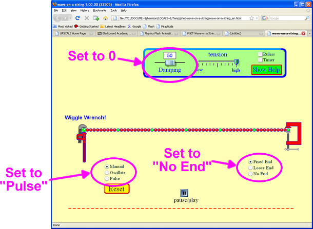
Download and open the Java applet wave-on-a-string_en.html.
-
Set the Damping to 0
-
Set the wave type to “Pulse”
-
Set the end to “No End” which will replace the clamp on the right side with an open window for the waves to go through.
Click on the Pulse button that will appear. Imagine you are standing right beside the window as the pulse goes out of it, measuring the displacement as a function of time as it goes by you. Sketch the displacement as a function of time.
-
Click on the Rulers control in the upper-right corner of the simulation. The rulers that appear can be moved with the mouse. Estimate the speed, width and amplitude of the wave pulse. Add labeled tick marks on the axes of the sketch of Part A.
This is a good time to experiment with different values of the Damping and tension. What happens as the Damping is increased? What happens as the tension in the string is decreased? You may wish to explore some of the other settings of the simulation too.
-
T
 he triangular pulse of Parts A and B was symmetric. Here is a plot of an asymmetric triangular pulse traveling from left to right. At the moment shown the time t = 0. The wave is traveling with a speed of 0.5 m/s. Sketch the displacement of the pulse at x = 0 as a function of time t as the pulse goes by. Include labeled tick marks on both the y and t axes.

-
Here is the same triangular pulse as Part B, but it is traveling from right to left at 0.5 m/s. At the moment shown the time t = 0. Sketch the displacement of the pulse at x = 0 as a function of time t as the pulse goes by. Include labeled tick marks on both the y and t axes. Compare to the sketch from Part C.

-
Here is a sinusoidal wave pulse traveling from left to right at v = 0.5 m/s. At the moment shown t = 0. Sketch the displacement of the pulse at x = 0 as a function of time t as the pulse goes by. Include labeled tick marks on both the y and t axes. What is the wavelength \(\lambda\) of the pulse? From your sketch what is the period T, frequency f, and angular frequency \(\omega\) of the sinusoidal pulse? What is the relation between \(\lambda\), f and v ?
-
H
 ere is a sinusoidal wave pulse traveling from right to left at v = 0.5 m/s. At the moment shown t = 0. Sketch the displacement of the pulse at x = 0 as a function of time t as the pulse goes by. Include labeled tick marks on both the y and t axes. What is the wavelength \(\lambda\) of the pulse? From your sketch what is the period T, frequency f, and angular frequency \(\omega\) of the sinusoidal pulse? What is the relation between \(\lambda\), f and v ?
 -
H
 ere is a sine wave traveling from left to right with v = 0.5 m/s. The wave extends to infinity in both directions along the x axis. At the moment shown the time t = 0. At the moment shown the displacement as a function of position is:
\(y(x,t=0)=0.1\sin(2\pi {x \over \lambda})\)
In your own words, explain the factor \(2\pi\) in the above equation. We can describe the displacement as the wave passes x = 0 either as \(y(x=0,t)=0.1\sin(2\pi{t \over T})\) or as \(y(x=0,t)=0.1\sin(-2\pi{t \over T})\). Which form is correct? Explain your own words. Write down a form of \(y(x,t)\) which is valid for all values of x and t. You may find the following Flash animation useful in visualizing this situation:
Activity 2
Here is a link to a simple little Flash animation of a plane wave traveling through two different mediums:
Open the animation.
-
At what rate do the wave fronts from the left strike the medium in the centre? What is the period, frequency, and angular frequency of the wave to the left of the medium in the centre?
-
For the medium in the centre, at what rate do the wave fronts leave the left-hand side? Is this the same as your answer to Part A? Explain. Do the wave fronts strike the right side of the medium in the centre at this same rate? What is the period, frequency, and angular frequency of the wave while it is traveling through the medium in the centre?
-
Click on the Show Ruler checkbox, and measure the wavelength of the wave traveling from the left to the medium in the centre. Measure the wavelength of the wave while it is traveling through the medium in the centre. Compare the ratio of the wave speed to the wavelength for these two cases. Explain your result.
-
The wave leaves the medium in the centre and travels off to the right. How do the period, frequency, angular frequency, and wavelength of the wave traveling to the right of the medium in the centre compare to the same quantities for the waves in the other regions?
Activity 3
In Activity 2 the waves strike the interface between the two mediums straight on, with zero angle of incidence. Here is a link to a Flash animation where the angle of incidence is not zero.
Open the animation.
-
At what rate do the wave fronts from the left strike the medium in the centre? Is the rate the same regardless of what vertical position you are considering? What is the period, frequency, and angular frequency of the wave to the left of the medium in the centre?
-
For the medium in the centre, at what rate do the wave fronts leave the left-hand side? Is this the same as your answer to Part A? Explain. Do the wave fronts strike the right side of the medium in the centre at this same rate? What is the period, frequency, and angular frequency of the wave while it is traveling through the medium in the centre?
-
How does the wavelength of the wave traveling from the left to the medium in the center compare to the wavelength of the wave while it is traveling through the medium in the centre? Show how you arrived at your answer.
-
T
 he wave leaves the medium in the centre and travels off to the right. How do the period, frequency, angular frequency, and wavelength of the wave traveling to the right of the medium in the centre compares to the same quantities for the waves in the other regions?
 -
The figure to the right shows a portion of two wave fronts of the animation. What is the relation between \(\theta_1\) and \(\theta_2\)? Notice that there are two right triangles in the figure with a common hypotenuse.
Activity 4
Here is a Flash animation of a molecular view of a sound wave traveling through the air:
Open the animation.
-
The bottom shows the motion of the air molecules. You may wish to imagine that the molecules are connected to their nearest neighbors by springs, which are not shown. There is a wave of increasing and decreasing density of the molecules. Is the wave moving to the right or to the left? Explain. Is the wave longitudinal or transverse? Explain.
-
Often instead of describing the wave as one of density we talk about a pressure wave. Does the higher density of molecules correspond to higher or lower pressure? Can you explain?
-
The top shows the displacement of the molecules from their equilibrium positions. Note that although the displacement value is plotted on the vertical axis, this actually represents displacement in the horizontal direction. It too is a wave, often called a displacement wave. Is the wave moving to the right or to the left? Explain. Is the wave longitudinal or transverse? Explain.
-
Use the step controls, pause the animation and position molecules 3 and 9 at their equilibrium position with molecule 6 at maximum displacement. The amplitude of the displacement wave is zero for molecules 3 and 9. Is the amplitude of the pressure wave at the position of molecule 3 also zero, or is it a maximum or a minimum? What about the pressure wave at the position of molecule 9?
-
Use the step controls to position molecules 3 and 9 at their equilibrium position with molecule 6 at minimum displacement. Is the amplitude of the pressure wave at the position of molecule 3 zero, or is it a maximum or a minimum? What about the pressure wave at the position of molecule 9?
-
From your results for Parts D and E, what is the phase angle between the pressure wave and the displacement wave?
Activity 5
-
Open the Java applet wave-on-a-string_en.html . Part A of Activity 1 shows a screen shot of the applet.
- Set the Damping to 0
- Set the wave type to “Oscillate”
- Set the end to “No End” which will replace the clamp on the right side with an open window for the waves to go through.
How does the amplitude of the wave change as it propagates down the string? Is this a one dimensional, two dimensional, or three dimensional wave? You may wish to look over Parts B and C before answering this question.
- A two dimensional wave, such as a water wave, is propagating away from its source equally in all directions. Assume damping is negligible. How does the amplitude of the wave change with distance from the source?
- A three dimensional wave, such as a sound wave, is propagating away from its source equally in all directions. Assume damping is negligible. How does the amplitude of the wave change with distance from the source?
- What physical principle or conservation law gives the answers to Parts A – C? Explain
Activity 6
-
Open the Java applet wave-on-a-string_en.html . Part A of Activity 1 shows a screen shot of the applet.
-
Set the Damping to 0
-
Set the wave type to “Pulse”
-
Leave the end in its default state of “Fixed End” which clamps the right side of the string with a C-clamp.
Click on the Pulse button. What is the behavior of the wave pulse when it is reflected by a fixed end?
-
Change the end of the string to “Loose End” which terminates the right hand side of the string with a frictionless loop around a vertical rod. Click on Reset and then on Pulse. What is the behavior of the wave pulse when it is reflected by a free end?
-
Set the end of the string back to “Fixed End,” click on Reset and then on Pulse. Use the pause/play button and then the step one to step the wave pulse through a complete reflection at one end of the string. There is a point where the wave pulse nearly disappears. Where did the wave go? Where did the wave’s energy go? Explain what is happening.
-
Set the end of the string back to “Loose End,” click on Reset and then on Pulse. Click on the Rulers control in the upper-right corner of the simulation. The rulers that appear can be moved with the mouse. Measure the maximum amplitude of the wave pulse; you may already have done this measurement in Activity 1 Part B. Use the pause/play button and then the step one to step the wave pulse through a complete reflection at one end of the string. There was a point where the amplitude of the wave at the position of the free end was large. Use the ruler to estimate its amplitude. Explain your result.
-
Set the end of the string back to “Fixed End.” Set the Damping to 10. Set the wave type to “Oscillate” and click on Reset. You will see a “standing wave” on the right hand side of the string. Use the pause/play button and then the step one to step the wave pulse through a complete reflection at the right end of the string. There is a point where the wave pulse near the right hand side nearly disappears. Where did the wave go? Explain what is happening.
-
Set the end of the string back to “Loose End,” click on Reset. You will once again see a “standing wave” on the right hand side of the string. Is there a difference between this standing wave and the one you saw in Part E? Explain. Is there a point where the wave displacement near the right hand side nearly disappears, as in Part E? Explain.
-
Set the end of the string back to “Fixed End.” Leave the wave type as “Oscillate.” Set the Damping to 0. Click on Reset. What happens? Explain.
Although we have used the wave on a string applet in Activities 1, 5, and now here, there is still lots more Physics that you can learn from it. You are invited to explore further.
Activity 7
“Music is a hidden practice of the soul, that does not know it is doing mathematics.” --Leibniz
If Pythagoras had a guitar, it might have looked like this:

We assume that Pythagoras was a large man, so the length of the strings from the bridge to the nut is 1 m, as shown.
The second string of six from the top is conventionally tuned to A two octaves below concert A. This is often written as A2, and has a frequency of 110 Hz.
The notes of an A scale starting at A2 are: A2 – B2 – C3# - D3 – E3 – F#3 – G#3 – A3. Here are the frequencies of these notes in a Pythagorean tuning; also shown are the frequencies of the notes in an equally tempered tuning which is more common today.
|
Note |
Pythagorean Tuning (Hz) |
Equally Tempered (Hz) |
|
A2 |
110.00 |
110.00 |
|
B2 |
123.75 |
123.47 |
|
C3# |
139.22 |
138.59 |
|
D3 |
146.67 |
146.83 |
|
E3 |
165.00 |
164.81 |
|
F3# |
185.63 |
185.00 |
|
G3# |
208.83 |
207.65 |
|
A3 |
220.00 |
220.00 |

You will need to know that, as discussed in the textbook, the speed of a traveling wave on string with tension Ts is
\(v_{string}=\sqrt{T_s \over \mu}\)
where \(\mu\) is the string’s mass-to-length ratio
\(\mu={m \over L}\)
Note that the speed is independent of the frequency.
To the right are shown the first four normal modes of a vibrating string.
Here is a link to a simple Flash animation that shows the actual motion of the string for the first three normal modes:
http://uoft.me/HFWStandingBoth
-
When the second string from the top is playing the note A2 = 110 Hz the frequency f of the first normal mode is also 110 Hz. What is the wavelength of the first normal mode? What is the speed of a traveling wave on the string? Explain why increasing the tension in the string increases the frequency of the note the string plays.
-
What is the wavelength of the second normal mode of the string? What is the frequency of the standing wave?
-
If you place your finger just to the right of the 12th fret the effective length of the string becomes 0.5 m, as shown in the figure. What is the wavelength of the first normal mode, and the frequency? What musical note is the string playing? How do your values compare to your result for Part B? Explain.
-
If you place your finger just to the right of the 7th fret the effective length of the string becomes 2/3 m, as shown in the figure. What is the wavelength of the first normal mode and the frequency? What musical note is the string playing? Explain.
-
Is there a pattern between the positions of the labeled frets in the figure of the guitar and the notes of the A scale in a Pythagorean tuning? What is the pattern? Are the lengths shown in the figure rational or irrational numbers? You may wish to know that if the guitar frets were set up to be equally tempered, except for the 12th fret the lengths would not be rational numbers.
-
As indicated in the table, the frequencies of the notes in a scale are slightly different in the Pythagorean tuning and the equally tempered tuning commonly used today. You may see if you can hear the difference by listening to a scale played with the Pythagorean tuning in the file Pythagorean.mid and a equally tempered tuning in EqualTempered.mid. You may also wish to explore further at: http://uoft.me/HFSTemperament .
Activity 8
At some position two sound waves have the form:
\(\begin{align*} D_1 &= a \sin(\omega_1 t) \\ D_2 &= a \sin(\omega_2 t) \end{align*}\)
They have the same amplitude a and different angular frequencies \(\omega_1\) and \(\omega_2\). In terms of the frequencies f1 and f2, the two waves have the form:
\(\begin{align*} D_1 &= a \sin(2\pi f_1 t) \\ D_2 &= a \sin(2\pi f_2 t) \end{align*}\)
The superposition of the two waves is:
\(\begin{align*} D_{\rm tot} &= D_1 + D_2 \\ &= A(t) \sin(\omega_{\rm avg} t) \end{align*}\)
where:
\(\begin{align*} \omega_{\rm avg} &= {\omega_1 + \omega_2 \over 2}\\ \\ A(t) &= 2a \cos(\omega_{\rm mod}t)\\ \\ \omega_{\rm mod} &= {|\omega_1-\omega_2| \over 2} \end{align*}\)
The amplitude of the wave, A(t), is modulated by the modulation angular frequency \(\omega_{\rm mod}\).
In terms of the frequencies the above relations become:
\(D_{\rm tot}=A(t)\sin(2\pi f_{\rm avg}t)\)
where:
\(\begin{align*} f_{\rm avg} &= {f_1 + f_2 \over 2}\\ \\ A(t) &= 2a \cos(2\pi f_{\rm mod}t)\\ \\ f_{\rm mod} &= {|f_1-f_2| \over 2} \end{align*}\)
-
If the frequencies of the two waves are close to each other you will perceive a wave with frequency favg whose amplitude is varying with a beat frequency fbeat = 2fmod. Say that the two waves have frequencies of 510 Hz and 512 Hz. Then you will hear a sound wave with frequency 511 Hz with a beat frequency of 2 Hz. In your own words, explain why the beat frequency is double the modulation frequency.
-
If the frequencies of the two waves are far apart, many but not all people will perceive an additional sound whose frequency is related to the difference in the two frequencies. Say that the two waves have frequencies of 220 Hz and 330 Hz. What is the frequency of the perceived sound? Explain. The audio file 330_220Hz_mix.mp3 is 15 seconds long. For the first 5 seconds, a 330 Hz sound is played. For the next 5 seconds, a 220 Hz sound is played. For the final 5 seconds, a mix two sounds are played together. Can anyone in your group perceive a third sound during the mixed part? This may only be possible for musical people. If one of you does perceive it, please describe it in your notebook: how does it compare to the first two sounds?
Activity 9
We can think of a sound wave two different ways:
-
A pressure wave. The pressure oscillates around atmospheric pressure.
-
A displacement wave. The displacements of the air molecules oscillate around their equilibrium positions.
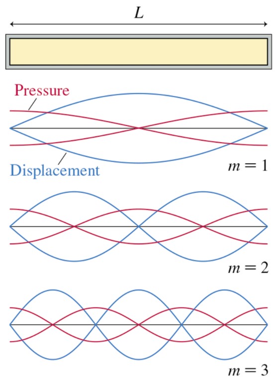
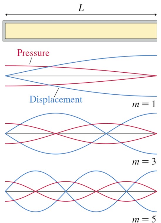
These two waves are 90 degrees out of phase: when one has a maximum or minimum the other is at zero amplitude. In a standing sound wave in a long narrow tube of air, an antinode of pressure occurs at a node of the displacement, and vice versa. An open end of a tube forces a node of the pressure wave (as it is open to ambient pressure), so there is an antinode of the displacement at an open end. A closed end of a tube forces a node of the displacement wave (as the air particles cannot oscillate left and right), so there is an antinode of the pressure at a closed end.
Here is Figure 17.15(a) from Knight, showing displacement and pressure graphs of the first three standing wave modes of a tube closed at both ends:
Here is Figure 17.15(c) from Knight, showing displacement and pressure graphs of the first three standing wave modes of a tube closed at the left end, and open at the right:
You will want to know that microphones measure the pressure wave. The approximate speed of sound in dry air at temperatures near room temperature is:
\(v_{\rm air} = (331.3 + 0.606\cdot T)\ {\rm m/s}\)
where T is the temperature of the air in Celsius (en.wikipedia.org/wiki/Speed_of_sound).
In this Activity you will set up standing sound waves in a tube filled with air and determine the speed of sound.
The Apparatus
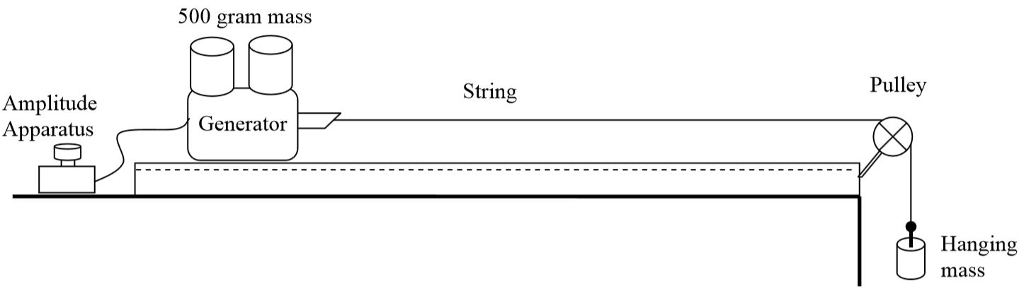
The apparatus is shown on the next page. The loudspeaker generates the sound wave. The rod inside the tube has a small microphone mounted on the end, so the sound wave inside the tube can be measured at different positions.

The figure below shows a close-up of the left side of the apparatus.
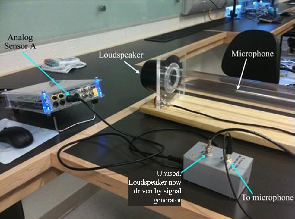
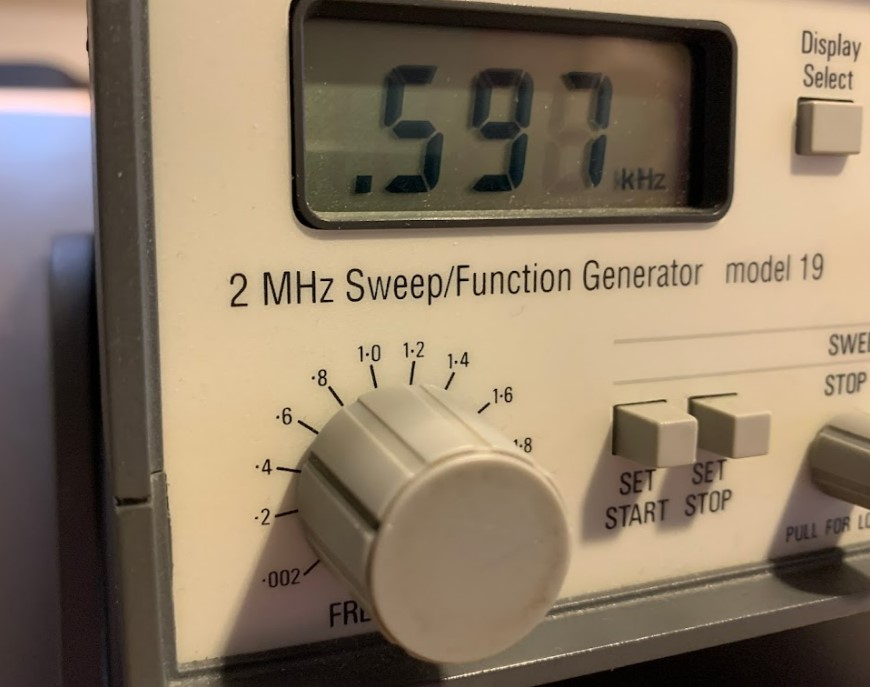
The gray box in the lower-right corner is the Sound Tube Microphone Amplifier. It is connected to the Analog Sensor A connection on the Data Acquisition Device. The connector labeled MIC is connected to the microphone. In our experiment, the loudspeaker is hooked to a separate signal generator. The signal generator has a course frequency adjustment on the front:
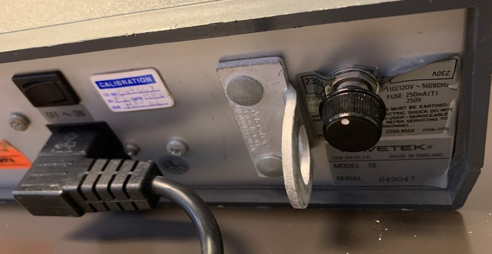
The signal generator has a fine-tuning frequency adjustment on the back, which has a range of +/- about 5% of the reading on the front:
The Software
The Speed of Sound Tube program measures the output from the microphone. [It was also originally designed to power the loudspeaker, but you will be using the separate signal generator to do that.] Click on Acquire Data in the upper-left corner. The button will turn green as shown. The plot on the right is what the microphone measures. It is a plot of Voltage versus time. The microphone voltage is proportional to the air pressure at the microphone position. You will be interested in the amplitude of the wave, which is about 1.5 V in the screen shot.

Getting a Standing Wave in the Tube
The most challenging part of this Activity is getting a standing wave set up in the tube. The actual tube differs from the ideal case because of a number of factors:
-
The cone of the loudspeaker is moving back and forth, so is only approximately a closed end.
-
The sound wave will reflect off the rod, the hole in the right hand side barrier, etc. This means that you are unlikely to measure nodes that have exactly zero amplitude. Instead the amplitude at the nodes will only be close to zero but will be much less than the amplitude at the antinodes.
Here are some tips for getting a standing wave. You may wish to repeat some of the steps as you get closer and closer to a good standing wave.
-
Step 1: When a standing wave is established, this is called resonance, and you will be able to hear that the sound that leaks out of the tube is louder than for a non-resonant condition.
-
Step 2: Place the microphone at the closed end of the tube. Slowly adjust the frequency so that you get a maximum amplitude from the microphone.
-
Step 3: Place the microphone at a node, and slowly adjust the frequency so that you get a minimum amplitude from the microphone.
For each standing wave that you study, be sure to record the range of frequencies for which you can not see any difference in the quality of the standing wave. This will determine the uncertainty in your value of the frequency.
Be careful not to push the Sound Sensor all the way into the speaker, as the speaker is made of paper!
Closed-Closed Tube
With the removable barrier in place so that the tube is effectively closed at both ends, get a standing wave in the tube. The stand that supports the rod straddles the metre stick. As you move the microphone from the nodes and antinodes of the standing wave, the distances between them can be determined by the position of the stand relative to the metre stick. HINT: To start, you might find that you can get an m=2 closed-closed mode at around 500 Hz. Note that the best standing wave will have maximum amplitude at its antinodes and minimum amplitude at its nodes. Once you have found the best frequency for a standing wave:
- What is the frequency of this standing wave? Estimate an uncertainty in the "best" frequency for this mode of standing wave.
- Measure the positions of all the nodes and antinodes in this pattern. Sketch the pattern. Which mode number, m, is this?
- The distance between adjacent nodes, or adjacent antinodes, is half the wavelength. From your position measurements, what do you estimate is the wavelength of this wave?
- The distance L is the effective length of the closed-closed tube \(L=\lambda m/2\). This is the distance between the outermost antinodes on either end. Based on your measurements of node and antinode positions, what is the effective L for this wave? [Check to make sure this seems to match the physical length of the tube.]
- Knowing the frequency and wavelength, what do you estimate is the speed of sound \(v=\lambda f\)?
Repeat steps A through E for two more standing wave modes at different frequencies, for a total of three closed-closed modes. Are the values of L consistent with each other? Are the values of the speed of sound consistent with each other? Knowing the temperature of the room, is the speed of sound what you would expect?
Open-Closed Tube
Remove the barrier from the end of the tube and establish a standing wave. Remember that only odd-numbered modes are possible in this configuration. HINT: To start, you might find that you can get an m=3 open-closed mode at around 450 Hz. Once you have found the best frequency for a standing wave:
- What is the frequency of this standing wave? Estimate an uncertainty in the "best" frequency for this mode of standing wave.
- Measure the positions of all the nodes and antinodes in this pattern. Sketch the pattern. Which mode number, m, is this? [Remember that m should be an odd integer.]
- The distance between adjacent nodes, or adjacent antinodes, is half the wavelength. From your position measurements, what do you estimate is the wavelength of this wave?
- The distance L is the effective length of the open-closed tube \(L=\lambda m/4\). This is the distance between the antinode on the left and the node on the right. What is L for this wave?
- Knowing the frequency and wavelength, what do you estimate is the speed of sound \(v=\lambda f\)?
Repeat steps A through E for two more standing wave modes at different frequencies, for a total of three open-closed modes. Is the average value of L you get here larger or smaller than it was for the closed-closed tube? Is the speed of sound you get here consistent with the closed-closed tube?
Activity 10
If the apparatus of Activity 9 were perfect, then when the tube is closed on both ends we would not hear any sound outside the tube. Similarly, if the air inside the tube were perfect, all molecule-molecule collisions would be perfectly elastic; this means that as a sound wave travels through the air none of its energy would be converted to heat energy of the air. However, neither the apparatus nor the air is perfect, The Quality Factor Q measures the degree of “perfection” of the system.
Say we have a standing wave when the frequency is f0. For frequencies close to the "resonant frequency" f0 the amplitude A of the sound wave at the position where there was an maximum in the pressure wave is given by:
\(A(f)=A_0{1 \over \sqrt{1+ Q^2\left( {f \over f_0} - {f_0 \over f}\right)^2}}\)
Note in the above that the amplitude A(f) is equal to A0 when the frequency f is equal to the resonant frequency.

The figure to the right shows A(f) for A0 equal to 1, Q equal 2, and for a resonant frequency of 50 Hz. Note that we have indicated the width of the curve where the maximum amplitude is \(1/\sqrt{2}\) times the maximum amplitude A0.
A nearly trivial amount of algebra shows that the amplitude A is \(1/\sqrt{2}\) times the maximum amplitude A0 for positive frequencies when the frequency is:
\(f={f_0 \over 2Q}(\sqrt{1+4Q^2} \pm 1)\)
Thus, if the width of the curve is \(\Delta f\) , then Q is:
\(Q={f_0 \over \Delta f}\)
Close the tube at both ends and adjust for a standing wave in the range of 200 Hz - 1 kHz. Place the microphone at a maximum in the pressure wave and take data for the amplitude as a function of frequency for frequencies close to the resonant frequency. Calculate the Quality Factor, Q, of the tube.
Activity 11: Waves on a String - First Experiment
Open the ‘Vibrating String’ software package. The apparatus should be setup similar to the picture below. For this activity make sure to use the nylon orange string. Set the amplitude apparatus at maximum by turning the black knob on the grey box.
ATTENTION: When the vibrating metal bar starts hitting the edges making a noise, turn the amplitude slightly down just until the noise stops.
- Hang a 100 gram mass on the end of the string near the pulley and set the frequency to very low. (e.g. 5 to 10 Hz). Gradually increase the frequency until the amplitude of the wave changes dramatically indicating that you have reached a resonance (maximum amplitude). How does the amplitudechange with the change in frequency (qualitative observation)? (Make sure the TA agrees that you have found a resonance. The most common problem for this activity is difficulty in noticing a resonance)
- Make a table in your lab book similar to the one below. Find four resonances (maximum amplitude) in a closed-closed end standing wave pattern, starting from the first resonance, and measure the distances between consecutive nodes to fill in the first two columns of your table. Be sure to draw the shape of each standing wave in your notebook.
|
Frequency (Hz) |
Distance between nodes (meters) |
Wavelength (meters) |
Speed of wave (m/s) |
|
| 1 | ||||
| 2 | ||||
| 3 | ||||
| 4 |
- Calculate the wavelength and wave speed for each of the standing waves to complete the table in your lab notebook. Find the average of these wave speeds.
- Determine the mass density of the string. Use this to calculate the theoretical wave speed value. Compare the average speed found above to the theoretically predicted speed value. Are they similar? Why or why not?
Activity 12: Waves on a String - Second Experiment
Open the ‘Vibrating String’ software package. The apparatus should be setup similar to the picture below. For this activity make sure to use the white/greenfishing line. Set the amplitude apparatus at maximum by turning the black knob on the grey box.
ATTENTION: When the vibrating metal bar starts hitting the edges making a noise, turn the amplitude slightly down just until the noise stops.
- Using hanging masses of 50 g, 100 g, 150 g, vary the frequency to give a closed-closed end standing wave pattern. Fill out the following table in your lab notebook:
| Mass (kg) |
Tension (N) |
Freq. (Hz) |
Distance between nodes (m) |
v (m/s) | v2 (m2/s2) |
- Make a plot of v2 vs.T (where T is the Tension) from the results in your table. What is the physical meaning of the slope?
- How does your measured slope compare with the theoretical value?
This Student Guide was originally written by David M. Harrison, Dept. of Physics, Univ. of Toronto in the Fall of 2008.
Activities 11 and 12 were written by Andrew Meyertholen in 2014.
The Java applet used in Activities 1, 5 and 6 was written by the Physics Education Technology (PhET) group at the University of Colorado, http://phet.colorado.edu/index.php. Retrieved November 9, 2008.
The figure of normal modes of a vibrating string in Activity 7 is slightly modified from Figure 21.22 of Randall D. Knight, Physics for Scientists and Engineers, 2nd edition (Pearson Addison-Wesley, 2008), pg. 640. The same figure is used in Activity 9.
The Pythagorean and equally tempered scales used in Activity 6 are from Wikipedia, http://en.wikipedia.org/wiki/Pythagorean_tuning. Retrieved November 15, 2008.
Activities 9 and 10 are based on a Student Guide written by David M. Harrison in October 1999 and revised in June 2001.
wave-on-a-string.jar was updated with a newer file from PhET and renamed wave-on-a-string_en.html in March 2018.