Catan 101

 

In this Module, we will consider dice. Although people have been gambling with dice and related apparatus since at least 3500 BCE, amazingly it was not until the mid-sixteenth century that Cardano began to discover the statistics of dice that we will think about here.

Although you will not be doing a huge amount of calculation as you go through this Module, you should use Python for both the calculations and making the histogram. If you do not know how to use Python now is a good time to begin learning this important tool. The Appendix has some tips on using Python for people who have some knowledge of the software, and some links to videos for beginners. After completing this Module, you will want to print the histogram that you will make, the window of the Python code and output of the code, and staple them into your notebook.

For an honest die with an honest roll, each of the six faces are equally likely to be facing up after the throw. Thus, for a pair of dice there are equally likely combinations. Of these combinations there is only one, 1-1 (“snake eyes”), whose sum is 2. Thus the probability of rolling a two is 1/36 = 0.03 = 3%. Similarly, there are two combinations whose sum is 3, 1-2 and 2-1, so the probability of rolling a three is 2/36. Table 1 summarises all of the possible combinations.

Probabilities for honest dice
Sum	Combinations	Number	Probability
2	1-1	1	1/36 = 0.03
3	1-2, 2-1	2	2/36 = 0.06
4	1-3, 3-1, 2-2	3	3/36 = 0.08
5	2-3, 3-2, 1-4, 4-1	4	4/36 = 0.11
6	2-4, 4-2, 1-5, 5-1, 3-3	5	5/36 = 0.14
7	3-4, 4-3, 2-5, 5-2, 1-6, 6-1	6	6/36 = 0.17
8	3-5, 5-3, 2-6, 6-2, 4-4	5	5/36 = 0.14
9	3-6, 6-3, 4-5, 5-4	4	4/36 = 0.11
10	4-6, 6-4, 5-5	3	3/36 = 0.08
11	5-6, 6-5	2	2/36 = 0.06
12	6-6	1	1/36 = 0.03

Table 1

A histogram is a convenient way to display numerical results. You have probably seen histograms of grade distributions on a test. If we roll a pair of dice 36 times and the results exactly match the above theoretical prediction, then a histogram of the results would look like the following:

 

 

 

 

 

 

 

 

Figure 1

 

---

    Activity 1

Roll a pair of dice 36 times, recording each result.  Each student in your team should roll the dice, for a total of 36 rolls.  (For example, if there are 3 of you in your team, you could each roll the dice 12 times, for a total of 36 dice rolls when you combine your data.) Make a histogram of the results. Qualitatively how do your results of this experiment compare to the theoretical prediction?

NOTE: In preparation for Activity 3, you should share your team's 36 dice-rolls with your instructor.  In Activity 3, your instructor will be combining all results to make a histogram of the rolls for all teams in your Practical Group.

---

 

Although this Module is part of a series on Uncertainty in Physical Measurements, the result of throwing the dice one time is certain: it is definitely a particular number. However, there is uncertainty associated with predicting the result of throwing the dice before you actually do it.

Your Instructors will collect the data for all the Teams’ results and combine them into a single dataset and histogram which will be shown on the screen later in this Module.

---

Questions

1. What is the probability of rolling a seven 10 times in a row?

2. Amazingly, you have rolled a seven 9 times in a row. What is the probability that the tenth roll will also come up with a seven?

---

A particularly powerful way of visualising the results shown Table 1 is to show the probability as a function of the sum. This is called a probability distribution, as shown in Figure 2. You will want to note that in the figure:

• We have added two “free” data points for sums of 1 and 13. Both of these are impossible, so their probabilities are 0.

• We have connected the dots.

• We have indicated the distance a from the maximum to the where the probability is 0 on the right. The quantity a is called the half-width of the distribution.

 

 

 

 

 

 

 

Figure 2

The line connecting the dots defines the probability distribution function (pdf) for rolling dice. This probability distribution function is triangular. We can write the pdf as:   

\(pdf{\rm (Sum)} = \begin{cases} \frac{1}{36}({\rm Sum}-1), & 1 \leq {\rm Sum} \leq 7 \\ \frac{1}{36}(13-{\rm Sum}), & 7 < {\rm Sum} \leq 13 \\ 0, & {\rm Otherwise} \end{cases}\)          (1)

We will see other examples of triangular probability distributions later, and will also learn about other shapes for probability distributions.

---

Questions

3. What is the sum of all of the probabilities given in Table 1?  Is this what you expected?

4. Imagine that you are about to roll the dice. What is the probability that the result will be 5, 6, 7, 8, or 9?

5. What is the total area under the pdf ? You can either integrate Eqn. 1 over the variable Sum, or you can use geometry and the fact that the area of a triangle is \(\frac{1}{2} \times base \times height\). How does your result compare to your answer to Question 3?

---

In your experiment you have collected 36 values of the result of throwing the dice. We will call each individual result S_i where i is an integer between 1 and 36. Then the mean or average of the 36 values is given the symbol and is given by:

\(\begin{eqnarray*} \bar{S}=\frac{\sum\limits^{36}_{i=1}S_i}{36} \end{eqnarray*}\)          (2)

For a symmetric probability distribution function, such as the triangular pdf that describes the dice, the theoretical value of the mean is the midpoint of the pdf, which in this case is 7.

Each individual measurement S_i may differ from the mean. The deviation d_i of each measurement from the mean is:

\(d_i \equiv S_i - \bar{S}\)            (3)

---

   Activity 2

Calculate the mean of the 36 dice rolls you performed in Activity 1. Compare your mean to the theoretical prediction of 7.

Calculate the deviations of each of your 36 individual measurements (dice rolls).

What the sum of the 36 deviations?  What is the theoretical prediction for the sum of the deviations?  Compare your sum to the theoretical prediction.

---

In Activity 2, you computed the sum of the deviations.  This turns out not to be a very useful number, as it is always expected to be near zero. If you want to find a single number which describes how close your measurements are to the mean value, it's better to sum of the square of the deviations. However, the value of the sum of the squares of the deviations depends on how many measurements were made. The standard way of dealing with this is the variance var, which normalises the sum by the number of measurements N – 1. The variance is defined as:

​\(\begin{eqnarray*} var\equiv \frac{\sum\limits^{N}_{i=1}(d_i)^2}{N-1} \end{eqnarray*}\)​       (4)

In general, for a triangular probability distribution function with data which matches the theoretical prediction, the variance can be shown to be:

\(\begin{eqnarray*} var = \frac{a^2}{6} \end{eqnarray*}\)        (5)

For the triangular probability distribution function of Figure 2, a = 6 and the variance is 6. Although we are not asking you to do so, it is fairly simple to show that this is correct for the data of Table 1.

You may wish to note that the definition of the variance, Eqn. 4, means that it can not be calculated for one measurement, since if N = 1 the denominator is zero: this is completely reasonable. Also for a large number of measurements the denominator  \(N - 1 \approx N\)and the variance is approximately the mean of the deviations squared.

---

   Questions

6. Three different Teams, A, B, and C, have done an experiment and made a histogram of their results:
   
   

 

 

 

 

 

 

 

 

 

 

 

 

 

 

 

 

 

 

 

 

 

 

 

 

 

 

 

 

 

 

 

Rank the variances of these three experiments. You do not need to do any calculations to do the ranking.

7. What is the variance of your experimental data from Activity 1?

---

   Activity 3

Do the combined results for all Teams, collected and shown by your Instructors, compare better or worse to the theoretical prediction than your experimental result for 36 rolls of the dice? Why do you think this is so?

To go a little deeper, let's focus on a specific question: "How many 7s did you roll, out of N rolls?"  The theoretical prediction is that about 16.7% of rolls should be 7s, and, for your team, N=36, so the number of 7s you rolled is expected to be near 6.  Did you get exactly 6 rolls that were sevens?  If not, do you suspect that your dice were faulty?  "Loaded dice" are dice that have been tampered with somehow by weighting or magnets so that they land with a specific side facing uwpwards more or less often than a fair die would.  If you did not roll exactly 6 sevens or of 36 rolls, would you suspect that your dice were loaded?  If you rolled 100% sevens after 100 rolls, would you suspect your dice were loaded?

This brings us to an insteresting question: How do you know when your measurements are "close enough" to the predicted result?  In real life you cannot expect exact agreement between experiment and theory, but it is important to know when the disagreement is big enough to mean there is a contradiction, meaning the theory is wrong or the experiment is flawed somehow.  

Devise a numerical method which, for a particular set of dice rolls, determines whether or not the number of 7s rolled is "close enough" to the prediction of 16.7% of N.   Note that there is no single correct answer to this. Some possible ways to do this is that if you roll n_7,exp sevens while the theoretical prediction of number of sevens is n_7,theory, then you can define “close enough” to be when the absolute value of the difference is less than or equal to some number C, i.e. |n_7,exp - n_7,theory| < C.  Or perhaps you decide it is more reasonable to define “close enough” to be that the difference is less than or equal to some fraction f of the theoretical value: |n_7,exp - n_7,theory| < f n_7,theory. You can perhaps devise other reasonable methods.  You might want to think about the fact that, the higher N is, the number of rolls, the closer you would expect the fraction of sevens to be 16.7% of N.   In the limit for which you rolled the dice an infinite number of times, you would expect to roll exactly 16.7% sevens, so "close enough" would be that  |n_7,exp - n_7,theory| = 0 in that case.

Use your method to quantitatively express how well your experiment’s results compare to the theoretical prediction, and how well the overall combined results compare to the theoretical prediction.  In both cases, according to your criterion, is the observed number of 7s rolled "close enough" to what is expected, or do the data suggest that someone is using loaded dice?

[Note, in Uncertainty Module 6 you will learn about a common method for determining whether a set of data is "close enough" to its prediction.]

 

---

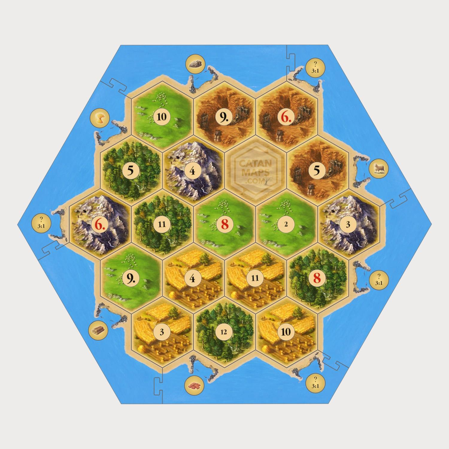Catan is a game in which the resources you earn are determined by the rolls of a pair of dice.  A player who chooses to build their resources near numbers with a high probability of being rolled has a better chance of earning more resources and winning the game!

 

---

Summary of Names, Symbols, and Formulae

Histogram: a graphical representation of the distribution of data. It is a series of rectangles whose height is proportional to the number of measurements in the range of values represented on the horizontal axis.

Probability Distribution: a distribution of probabilities.

Half-width a: one-half of the total width of a probability distribution.

Probability Distribution Function (pdf): a function representing a probability distribution.

For N repeated measurements: x₁, x₂, x₃, … , x_N:

Mean or average \(\begin{eqnarray*} \bar{x} = \frac{\sum\limits_{i=1}^N x_i}{N} \end{eqnarray*}\)

Deviation  \(d_i = x_i - \bar{x}\)

Variance ​\(\begin{eqnarray*} var\equiv \frac{\sum\limits^{N}_{i=1}(d_i)^2}{N-1} \end{eqnarray*}\)​

For a triangular pdf of half-width a   ​\(\begin{eqnarray*} var = \frac{a^2}{6} \end{eqnarray*}\)​

 

Appendix

If you are already reasonably familiar with Python then we will begin by giving you some tips on using it with this Module. For relative beginners, we have prepared a series of tutorials to get you started in Python, for which a link is provided below. Here are the tips:

• After starting Spyder, it is a good idea to begin your program with the following two lines, which load many useful functions:

  from pylab import *
  from numpy import *

  Although you can write down the result of rolling the dice 36 times, and then transfer the data to the program, you can just as easily enter the data as you go. Say your first three rolls are a 4, a 6, and a 12. Then the next line of the program could be:

• dice = [4, 6, 12,

  Then as you continue to roll the dice, enter each result followed by a comma. For the last 36^th roll, do not follow the number by a comma but instead by a right square bracket ].

• Note that the name dice is arbitrary: you can call it anything that you wish; below we will assume that you have used the name dice. Also, in case something goes wrong, you should also enter the data by hand into your notebook as you take it.
  To make a histogram of the dice data: 

  hist(dice, bins = 11, range = (2, 12))
  show()

   

• To print the histogram, a simple method is from the window containing the histogram save the image to a file, and then open the file with a browser and use the browser’s print command.
  The command to calculate the mean is mean(data). To calculate the deviations, you will need to store the result in a variable: the name of the variable is arbitrary but we will use the name mean. So these lines calculate the mean, stores the result, and prints it:

  mean_value = mean(dice)
  print("average:", mean_value)

   

• Note the underscore in the variable name mean_value.
  
  Python is pretty smart about names. The following lines also work:

  mean = mean(dice)
  print("mean:", mean)

  Here the string mean is used three ways in the above two lines: one is an arbitrary variable name, the second is the name of the function that does the calculation, and the third is the arbitrary label inside the quotes in the print command. However, “overloading the namespace” is considered to be poor programming practice and can occasionally lead to problems: the first form of calculating and printing the mean is preferred.

• To calculate the deviations, you will subtract the variable mean from the data. To do the calculation, store the result in a variable named devs, and print the deviations:

  devs = dice - mean
  print("deviations:", devs)

• To calculate and print the sum of the deviations: 

  print("sum of deviations:", sum(devs))

  The Python routine to calculate variances is called var. By default it defines the variance as: which is not quite the same as Eqn. 4. To use the definition of Eqn. 4:

  print("variance:", var(dice, ddof = 1))

  The name ddof stands for delta degrees of freedom. You will learn more about this name in Module 5.

• You can also calculate the variance yourself with: 

  print("brute force var:", sum(devs**2)/(len(dice) - 1))

  To print the output window, save it as a file and then use the File / Print Window command available in the window itself. To print the input window, you will also need to save it as a file and use File / Print Window.

 

Here is a four-part Tutorial Series on using Python for physics: http://compwiki.physics.utoronto.ca/Getting+Started+(Fall+2017) .

 

This Guide was written by David M. Harrison, Dept. of Physics, Univ. of Toronto, September 2013.