Uncertainties Introduction
Table of contents
1. Introduction to Repeated Measurements
For a finite number of measurements we can estimate the mean:
\(\bar{x} = {1 \over N}\sum \limits_{i=1}^N x_i\ \) (1)
We can also use the data to estimate the standard deviation:
\(\begin{align*} \sigma & = \sqrt{ {1 \over N-1} \sum_{i=1}^N(x_i-\bar{x})^2} \end{align*}\) (2)
For any individual measurement xi, the estimated uncertainty in the value of the measurand is:
\(u(x_i)=\sigma\) (3)
Note that this is not the uncertainty in the value of the estimated mean \(\bar{x}\): it is the uncertainty in each individual measurand xi. For a Gaussian pdf, the area under the curve between \(\mu - \sigma\) and \(\mu + \sigma\) is 0.68. Therefore it is reasonable to assume that the probability that for a single measurement xi the true value of \(\bar{x}\) is within \(\sigma\) of xi is 0.68. Put another way, if you choose one of the measurements of the distance xi at random, there is a 68% chance that it is within one standard deviation of the true value of the position.
Since this uncertainty arises from the scatter of values due to various random effects, this type of uncertainty is often called statistical.
2. Significant Figures Involving Uncertainties
When uncertainties for quantities are given, the rules for significant figures are:
- Uncertainties should be specified to one, or at most two significant figures.
- The most precise column in the number for the uncertainty should also be the most precise column in the number for the value.
So if the uncertainty is specified to the 1/100th column, the quantity itself should also be specified to the 1/100th column.
 Question 1
Express the following quantities to the correct number of significant figures:
- 25.052 ± 1.502
- 92 ± 3.14159
- 0.0530854 ± 0.012194
- \(3.2478 \times 10^{-6} \pm 1.9518 \times 10^{-7}\)
- \(6.674076391 \times 10^{-11} \pm 3.10895 \times 10^{-15}\)
 You may have seen other definitions and ways of dealing with significant figures elsewhere. For experimentally determined quantities, those definitions and properties are not appropriate! Use these rules instead!
3. Propagation of Uncertainties
Say we have measured some quantity x with uncertainty u(x) and a quantity y with uncertainty u(y) and wish to combine them to get a value z with uncertainty u(z). We need the combination to preserve the probabilities associated with the uncertainties in x and y. We will consider a number of ways of combining the quantities.
Addition or Subtraction
If z = x + y or z = x – y then the uncertainties are combined in quadrature:
\(u(z)=\sqrt{u(x)^2 + u(y)^2}\) (4)
Multiplication or Division
If z = xy or z = x/y then the fractional uncertainties are combined in quadrature:
\(\begin{eqnarray*} {u(z) \over |z|} = \sqrt{\left({u(x) \over x}\right)^2 + \left({u(y) \over y}\right)^2} \end{eqnarray*}\) (5)
Multiplication by a Constant
If z = ax, where a is a constant known to a large number of significant figures, then the uncertainty in z is given by Eqn. 5 with the uncertainty in a, u(a) = 0. So:
\(u(z) = |a| u(x)\) (6)
Raising to a Power
If z = xn then:
\(u(z) = n x^{(n-1)}u(x)\) (7)
which can also be written in terms of the fractional uncertainties:
\(\begin{eqnarray*} {u(z) \over z} = n{u(x) \over x} \end{eqnarray*}\) (8)
Say you are squaring x, so \(z = x^2 = x \times x\). You may be tempted to use Eqn 5 for multiplication and division, but this is incorrect: Eqn 5 assumes that the uncertainties in the quantities x and y are independent of each other. Here there is only one quantity, x.
Be sure to remember that in call cases u(z) defines the significant figures in z.
The General Case
In general z is some function of x and y, z = f(x, y). The uncertainty in z is given by partial derivatives:
\(u(z)=\sqrt{\left[ {\partial f(x,y) \over \partial x}u(x)\right]^2+\left[ {\partial f(x,y) \over \partial y}u(y)\right]^2}\) (9)
Eqns. 4 – 8 are just applications of Eqn. 9 for various functions.
Question 2
Eqn. 7 may look familiar to you. What does it look like? Hint: try writing u(z) as dz and u(x) as dx.
Question 3
You measure a quantity to be \(3 \pm 1\) and another quantity to be \(70 \pm 2\) . What is the uncertainty in the sum to one significant figure? Does the uncertainty in the value of 3 have any effect on the uncertainty in the sum to one significant figure? Write down the sum \(\pm\) its uncertainty to the correct number of significant figures. Remember that the uncertainty only has one or at the very most two digits that really are significant, and that the uncertainty determines the number of digits in the value that are significant.
4. The Uncertainty in the Mean
We have seen that for N repeated measurements, x1, x2, … , xN, the statistical uncertainty in each individual measurand xi is the standard deviation \(\sigma\). We now know enough to determine the uncertainty in the estimated mean, \(u(\bar{x})\). The estimated mean is given by:
\(\begin{align*} \bar{x} & = {1 \over N} \sum_{i=1}^N x_i \\ & = { [x_1 \pm u(x_1)] + [x_2 \pm u(x_2)] + ... + [x_N \pm u(x_N)]\over N} \end{align*}\) (10)
But the uncertainty in each individual measurement is the same, which we will call u(x): \(u(x) \equiv u(x_1) = u(x_2) = ... = u(x_N)\). Combining all the uncertainties in the numerator in quadrature gives:
\(\begin{eqnarray*} \bar{x} = { (x_1 + x_2 + ... + x_N) \pm \sqrt{N} u(x) \over N} \end{eqnarray*}\) (11)
The numerator is divided by the constant N, so from Eqn. 5:
\(\begin{eqnarray*} \bar{x} = { (x_1 + x_2 + ... + x_N) \over N} \pm { u(x) \over \sqrt{N}} \end{eqnarray*}\) (12)
or:
\(\begin{eqnarray*} u(\bar{x})={u(x) \over \sqrt{N} } \end{eqnarray*}\) (13)
So repeating a measurement N times reduces the statistical uncertainty in the mean by a factor of \(1 / \sqrt{N}\) times the uncertainty in each individual measurement. So repeating a measurement 4 times reduces the uncertainty by a factor of ½.
The fact that the uncertainty in the mean is less than the uncertainty in each individual measurement should not be a surprise: we repeat measurements precisely so that we increase our knowledge of the true value of what we are measuring, i.e. in order to reduce its uncertainty.
5. Activities
 Activity 1
Imagine that you have measured the time for a pendulum to undergo five oscillations, t5, with a digital stopwatch. You repeat the measurements 4 times, and the data are:
|
t5 (s) |
|
7.53 |
|
7.38 |
|
7.47 |
|
7.43 |
What is the mean of the four measurements of t5, and uncertainty in this mean value? Express your final result as \(\bar{t_5} \pm u(\bar{t_5})\) . Be sure to use the rules for significant figures when uncertainties are involved.
 Activity 2
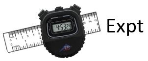
Using the supplied digital stopwatch, try to start it and then stop it at exactly 2.00 s. It may take a few tries to get better at this. After practicing, repeat a few times. All members of the Team should do this, so you may end up with about 15 or 20 values. Report all the values in your notebook. Just by looking at the data and without doing any calculations, choose a value of u such that most but not necessarily all measurements are between 2.00 – u and 2.00 + u.
 Activity 3
 You are supplied with a standard 8 ½ by 11 inch sheet of paper and a digital stopwatch. Hold the paper horizontally at shoulder height and release it. Use your stopwatch app to measure the time t it takes the paper to reach the floor. Repeat for a total of 20 times for your whole pod, excluding trials where the paper strikes something as it falls.
Make a histogram of the results of your experiment. You will need to decide the range and how many bins to use in making the histogram. The decision is based somewhat on the scatter of values. In the Appendix there is some guidance about how to use Python using the Spyder editor on your pod computer to enter the data and make a historgram.
Is it reasonable to assume that the scatter of values of t can be described by a Gaussian probability distribution function?
Assuming Gaussian statistics are valide, what is the estimated statistical uncertainty in each measurement of t, i.e. the estimated standard deviation?
In Activity 2 you estimated an uncertainty in the individual time measurements due to human reaction times, call it \(u_{\rm reaction}(t_i)\). You have just found another uncertainty in the individual measurements, the one due do the random fluctuations in the times you measured for different trials; we will call this the statistical uncertainty \(u_{\rm statistical}(t_i)\) . It is reasonable to combine these two uncertainties in quadrature, the square root of the sum of the squares, to estimate the total uncertainty in each individual measurement.
Do the calculation of combining these two uncertainties. Remember from Question 3 that if one uncertainty is much smaller than the other, than when combining them in quadrature to only 1 or 2 significant figures the smaller value has negligible effect on the combination, and sometimes it is not even worth the effort of doing the calculation. Does the smaller of the uncertainties being combined here have a significant effect on the value of the combination?
Can you think of any other uncertainties, such as the reading uncertainty of a digital instrument or the accuracy of the stopwatch, which might have a significant effect on the total uncertainty in your measurements of ti? If so, calculate their effects.
Finally, what is estimated mean time for the paper to reach the floor, and what is the uncertainty in this time? Present your final result as \(\bar{t} \pm u(\bar{t})\) .
Appendix
If you are already reasonably familiar with Python then we will begin by giving you some tips on using it with this Module. For relative beginners, we have prepared a series of tutorials to get you started in Python, for which a link is provided below. Here are the tips:
-
After starting Spyder, it is a good idea to begin your program with the following two lines, which load many useful functions:
from pylab import *
from numpy import *
Although you can write down the result of rolling the dice 36 times, and then transfer the data to the program, you can just as easily enter the data as you go. Say your first three measurements are 2.12, 1.96 and 2.01. Then the next line of the program could be:
-
meas = [2.12, 1.96, 2.01]Then as you continue to make measurements, enter each result followed by a comma. For the measurement, do not follow the number by a comma but instead by a right square bracket].
-
Note that the name meas is arbitrary: you can call it anything that you wish; below we will assume that you have used the name meas. Also, in case something goes wrong, you should also enter the data by hand into your notebook as you take it.
To make a histogram of the meas data:hist(meas, bins = 11, range = (1.5, 2.5)) show() -
To print the histogram, a simple method is from the window containing the histogram save the image to a file, and then open the file with a browser and use the browser’s print command.
The command to calculate the mean is mean(data). To calculate the deviations, you will need to store the result in a variable: the name of the variable is arbitrary but we will use the name mean. So these lines calculate the mean, stores the result, and prints it:mean_value = mean(meas) print("average:", mean_value) -
Note the underscore in the variable name mean_value.
-
To calculate the deviations, you will subtract the variable mean from the data. To do the calculation, store the result in a variable named devs, and print the deviations:
devs = meas - mean_value print("deviations:", devs) -
To calculate and print the sum of the deviations:
print("sum of deviations:", sum(devs))The Python routine to calculate variances is called var. By default it defines the variance as: which is not quite the same as Eqn. 2. To use the definition of Eqn. 2:
The name ddof stands for delta degrees of freedom. You will learn more about this name in Module 5.print("variance:", var(meas, ddof = 1)) -
You can also calculate the variance yourself with:
print("brute force var:", sum(devs**2)/(len(meas) - 1))To print the output window, save it as a file and then use the File / Print Window command available in the window itself. To print the input window, you will also need to save it as a file and use File / Print Window.
Based on a guide originally written by David M. Harrison, Dept. of Physics, Univ. of Toronto, September 2013.