Mechanics Module 4 Student Guide

  Activity 1

Note:in this Activity you will be using a Force Sensor with a spring bumper mounted on it. Please do not adjust the bumper. If you think it needs adjustment contact your Instructor.

Setup notes:

• Make sure the Track is level.

• The Motion Sensor should be mounted on the end of the Track closest to the wall and connected to the Data Acquisition Device.

• A C-clamp should be attached about half-way down the track for the cart to collide with.

• The Force Sensor with the spring bumper attached should be mounted on the Cart. The spring bumper should not be loose, but it also must not be over-tightened, or the mounting could be damaged. Speak to a TA if you think the bumper is not attached properly. Measure the total mass of the Cart and Force Sensor, not including the wire, which shouldn't be part of the motion.

• Place the Cart on the Track with the bumper facing the C-clamp. Connect the Force Sensor to the Data Acquisition Device. Press the Tare button on the Force Sensor to zero its readings.

• Run the Cart up and down the Track a few times to warm up the bearings in the wheels.

• Set the sample rate for the Motion Sensor to 50 samples per second. 

You will want to “trim” your data after you have collected it using the tools provided by the software. Appendix A is a brief discussion of things you may wish to do. For full details consult the manuals for the Force Sensor and the Motion Sensor, which are available at: http://www.upscale.utoronto.ca/Practicals/Manuals/Manuals.html .

Now the Activities:

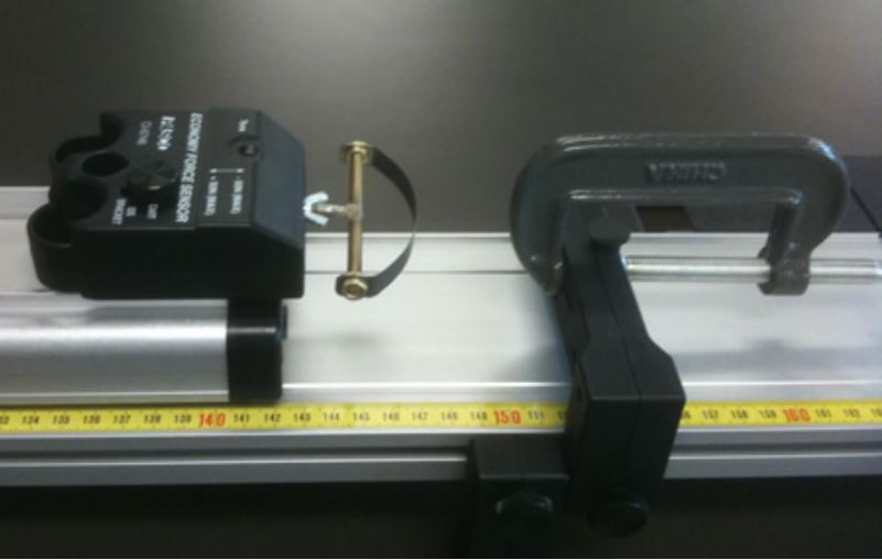
1. You want the spring bumper on the Force Sensor to collide with the C-clamp. The Cart will drag the wire connecting the Force Sensor to the DAQ board; make sure it is as free to move as possible. You may need to adjust the position of the Track and/or C-clamp to get a nice “clean” collision. Here is a photograph of the cart and the C-clamp.

 

 

 

2. Take data on the speed versus time using the Motion Sensor and force versus time using the Force Sensor from a second or so before the collision to a second or so after the collision. Remember to press the Tare button on the Force Sensor just before taking your data. NOTE: Every collision is different!  So you MUST simultaneously record the force data and the motion sensor data, and analyze a single collision.  You cannot combine force data from one collision with the motion sensor data from a different collision!

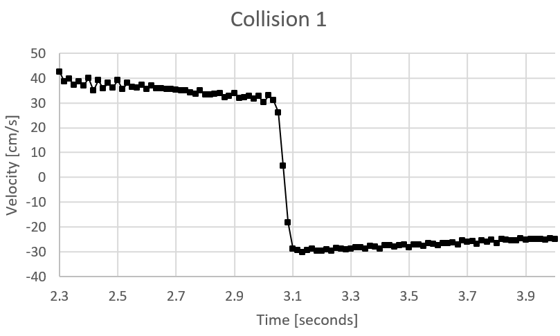
3. From the speed versus time data, what is the momentum of the Cart plus Force Sensor just before the collision? What is the momentum just after the collision? Choose your coordinate system so that the velocity of the Cart before the collision is in the positive direction.

4. What is the change in the momentum of the Cart plus Force Sensor from just before the collision to just after? (As always, include uncertainty.)

5. From the force-time data, estimate the area under the force-time graph. You can set up two vertical lines on the Labview Software called Cursor0 and Cursor1, and click the "Integrate" button to obtain the area under the curve between the two cursors, in Newton-seconds (N s).   Be sure to move the cursors around a bit, and estimate the uncertaintly in your result.
   Compare your result to what you found in Part D. Do your results agree within the measurement uncertainties?  REMEMBER: If you want to repeat the experiment, you must simultaneously run the force sensor and the motion sensor each time so that you are always analyzing the same collision.  Don't compare data from different collisions, as your initial velocities will be different.
    

 

In preparation for Activity 2, export your speed-time data from Activity 1 into a file on the computer, by going to "File" and "Velocity Data Set", click "Save". You will need to choose a name for your file, such as "velocity data collision 1".

   Activity 2

The Physics presented in textbooks almost always deals with ideal cases. For example, in that context we often say “ignore air resistance” or “assume that friction is negligible.” In the real world, often these idealizations are not correct.

For example, we know that there is always friction between the Cart and the Track. In Activity 1, there was additional “friction” because the Cart was dragging the wire of the Force Sensor, and the effect of these two forces is easily seen in the data.  Notice that the velocity is not quite constant before or after the collision.

These extra forces are in the opposite direction to the motion of the Cart, so always slow down the magnitude of the velocity, regardless of whether the velocity is a positive or negative number.  It is also true that the collision of the spring bumper with the C-clamp is not perfectly elastic, so the magnitude of the velocity is less just after the collision than just before.  We would like to eliminate the friction effects, and find the velocity of the cart just before the collision, and just after, in order to best compare with the impulse measured by the Force Sensor.

1. Use Excel to make a Chart of velocity versus time, like the figure above.  [Refer to Appendix B below if you are new to Excel.]  Estimate the time of the "centre" of the collision, when the impulse is maximum.  This we will call t_coll. 

2. Make a second chart that only includes velocities before the effects of the bumper.  Add a trendline, make it "linear", and display the equation for this trendline on your chart.  Use the equation to predict the velocity the cart would have had at the moment t_coll, if the collision had not occurred.  This is v_i, the initial velocity, just before the collision.

3. Make a third chart that only includes velocities after the effects of the bumper.  Add a trendline, make it "linear", and display the equation for this trendline on your chart.  Use the equation to predict the velocity the cart would have had at the moment t_coll, if the collision had not occurred.  This is v_f, the final velocity, just after the collision.

4. This should give you a slightly better estimate for the change in velocity due to the collision.  How does this compare to the impulse you measured for this particular collision?

5. Considering your data and your experience with these Carts, which force do you think is largest, friction or dragging the wire?

 

   Activity 3

You are asleep in your room, but a fire has broken out in the hall and smoke is pouring in through the partially open door. You need to close the door as soon as possible. The room is so messy you cannot get to the door. You have a ball of clay and a super ball, each with the same mass. If you throw the clay at the door it will stick to it; if you throw the super ball at the door it will bounce off. You only have time to throw one thing at the door.

1. Which should your throw at the door, the clay or the super ball? Explain.

2. Which ball will experience the largest impulse during the collision?

3. From Newton’s 3^rd Law the impulse that the door exerts on the ball during the collision is equal in magnitude although opposite in direction to the impulse the ball exerts on the door. Which ball exerts the largest impulse on the door?

 

    Activity 4

 

Three identical balls slide on a table and hit a block that is fixed to the table. In the figures we are looking down from above. In each case the ball is going at the same speed before it hits the block.

 

 

 

 

Rank in order from the largest to the smallest the magnitude of the force exerted on the block by the ball.

 

 

 

 

 

    Activity 5

An air track is similar to the Track you have been using in the Practicals. The track has small holes drilled in it, and air blows out of the holes. Thus the carts for the air track float on the air and there is extremely low friction between the cart and the track. An animation of an air track is at:

http://uoft.me/HFMAirTrack

There are six possible collisions that may be simulated: three different values for the mass of one of the carts, with elastic “bouncy” and inelastic “sticky” collisions for each value of the mass.

1. The momentum \(\vec{p} = m\vec{v}\) is also called the quantity of motion and sometimes just the inertia. For Newton momentum was central to his thinking about dynamics. Use the animation to determine if the total momentum of the carts is conserved before and after each of the six possible collisions.

2. For Leibniz, a contemporary and rival of Newton, momentum was not central to his thinking. Instead he concentrated on the quantity \(mv^2\), which he called the vis viva (literally “living force”). Use the animation to determine if the total vis viva of the carts is conserved before and after each of the six possible collisions.

3. Which concept, momentum or vis viva, appears to be the most fundamental?

 

Appendix A – “Trimming” the Data

For the data collected by the Motion Sensor, you will want to select the velocity versus time data for times just before the collision to just after the collision. In the Analyze tab use the mouse to grab the cursors in the left-hand plot of Distance versus Sample to select the desired region. The graphs to the right of this plot show only the data between the two cursors.

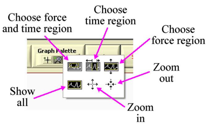
For the Force Sensor data, you will similarly want to look at the force versus time data for times just before to just after the collision. In the upper-right corner of the Force Sensor vi is a item labeled Graph Palette. Clicking on the middle of the three buttons in the palette shows a pull-down menu as shown. Select Choose time region and “paint” in a region of time values on the graph to display only force-time data for the selected region. The Show all item undoes any previous selections and displays all the data.

In calculating the impulse \(J = \int Fdt\) from the force-time data you can use the Integrate button on the front panel of the Force Sensor vi. This function calculates the area under the curve between the two cursors, which are called Cursor 0 and Cursor 1. To move the cursors with the mouse, choose the left-hand button in the Graph Palette, whose icon is the crossed lines that can be seen in the above figure.

 

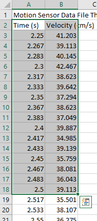
Appendix B – Using Excel

Open Microsoft Excel and click File- Open.  You will need to Browse folders to find the data that was saved by the Labview Motion Sensor.  If you don't see your data, you might need to click on "All Excel Files" and change it to "All Files", as Labview only saves text files.  Choose your data, click Open, choose "Delmited", Next, "Tab" delimiters, Next and Finish.  To insert a chart, first click on the data you want to graph:

Next click the Insert tab, and under Charts choose "Scatter" with smooth lines and markers.

Note that you can insert multiple charts by selecting the specific data you wish to graph.

You can click the + button to add chart elements such as Axes Titles, which you can edit. 

You can click on an axis, and choose "Axis options" to change the bounds so the data fill the chart.

If you click on the chart and then click File - Print, it should send only this chart to the printer, which you can then staple into your Notebook.

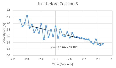
If your data appear to be a straight line, you can click the + and select Trendline.  You can also go to More Options, and choose to "Display Equation on chart". If you have a linear trendline it should give you an equation in the format y = mx + b, where x represents time, y is velocity in cm/s, m is the slope (representing friction) and b is the y-intercept (representing the velocity at time t=0).

 

 

This Guide was written in July 2007 by David M. Harrison, Dept. of Physics, Univ. of Toronto. Some parts are based on Priscilla W. Laws et al., Workshop Physics Activity Guide (John Wiley, 2004), Unit 8.
Modified by Lilian Leung in October 2021.  Modified by Jason Harlow in Oct.2023.