Analog Instruments

In this Module we will consider instruments with an analog readout. You will be using a ruler to measure the diameter of a coin.

Imagine we are measuring some position with a ruler. A portion of the ruler that measures the position in cm and the point representing the position are shown below.

 

Figure 1

Assume for now that the ruler is perfectly constructed. So what is the value of the position?

This is a tough question. Certainly it is greater than 18 cm and less than 19 cm. It is also certainly greater then 18.1 cm and less than 18.9 cm. Perhaps it is reasonable to say that the position is between 18.3 cm and 18.5 cm, although you may reasonably decide that it is between a narrower or wider range of values than these. We’ll assume the position is between 18.3 and 18.5 for now. The probability that the position is either 18.3 or 18.5 cm are both zero; it is greater than 18.3 and less than 18.5. The most probable value for the position is half-way between 18.3 and 18.5, i.e. 18.4 cm. What about a value of 18.35 cm? This is certainly possible, although it is less likely than that it is 18.4.

Therefore, it is reasonable to approximate this measurement with a probability distribution function pdf that is triangular, as shown in Figure 2.

 

 

 

 

 

 

 

Figure 2

 

---

  Questions

1. What is the value of p in Figure 2?

2. What is the value of the measurand, i.e. the position, and its uncertainty? You will want to remember:

   • From Module 1, that the variance of a triangular distribution of width a is \(a^2/6\). There we considered integer values of the measurand, the outcome of rolling a pair of dice. By using integral calculus it can be shown that the variance is also equal to this value for continuous values of the measurand.

   • From Module 2, that the uncertainty u is equal to the standard deviation \(\sigma\) which is equal to the square root of the variance.

---

 

In Module 2 we learned that for a rectangular pdf the probability that the value of the quantity being measured is within \(\pm u\) of the value of the measurand is 0.58.

For a triangular pdf as in Figure 2 we have shaded the region between 18.4 – u and 18.4 + u where u is the correct answer to the uncertainty found in Question 2. It is not hard to show that the shaded region has an area of 0.65. Therefore the probability that the true distance is within  \(\pm u\) of the value of 18.40 is 0.65.

 

  Activity 1

Suppose that you measure the same position that we have been considering but with a different ruler, as shown in Figure 3.

Figure 3

Perhaps the extra scale divisions of this ruler will guide your eyes and allow you to make a different estimate of the triangular pdf of the measurement. So for this measurement what is the position and its uncertainty?

Note that assigning the half-width a of the triangular pdf is subjective: it is your eyes and the resolution of the figure that you are looking at that determines the answer. Also, there is always a trade-off involved is assigning a value to a. You want it to be large enough that the probability that the value is \(\pm a\) away from the central value is essentially zero. However, you also want a to be as small as possible, so that the corresponding uncertainty is as small as possible. This trade-off is always true in assigning a value to a.

How does your answer compare to your answer to question 2?

Hint	You may have seen other rules for deciding how well you can read an analog instrument. Often these rules are related to the values of scale markings on the instrument. Here we will show that those other rules are wrong.
Consider the measurement of a voltage with a voltmeter, a shown to the right. Perhaps it is reasonable to say that the voltage is between 7.30 and 7.40 Volts.
Here is the same measurement, except that the person doing the measurement needs to put on their glasses. It seems fairly obvious that the uncertainty in the result of this measurement is larger than the previous one.
The point is that there is no fixed rule to determine the width of the probability distribution function or the uncertainty in the measurement. For example, in Activity 1 it is your eyes and the resolution of the screen or printout displaying the figure that determines your answers.

 

   Activity 2

Part A: 

Measure the diameter of a coin with the supplied digital caliper. Determine the uncertainty in your measurement. Write down the diameter of the coin as the measurand the uncertainty.

Part B:

Using the supplied ruler, measure the diameter of the same coin and calculate the uncertainty in your measurement. 

Note that you will do two measurements for the positions of opposite sides of the coin, and will subtract them to calculate the diameter. As shown in the figure, this is true even if you try to put one edge of the coin on the 0 mark: there will still be an uncertainty in the value of 0. Note the rulers shown in the figure are not to scale.

What is the value of the diameter and its uncertainty?

Part C:

How does your result in Part A compare to your result in Part B? A nice way to answer this question is to subtract the smallest value of the measurand from the largest one. Is the result zero within the combined uncertainty?

 

Hint

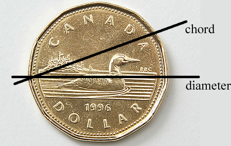
There is another issue with your measurement of the diameter of a coin: perhaps the ruler is not measuring the actual diameter but only the length of a chord because the ruler was not oriented quite correctly. This does not give an uncertainty in the result, it is an error. This type of error is called a systematic error. We will discuss how to deal with systematic errors in more detail later.

---

    Question

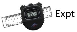
3. A mass on a string is oscillating back and forth, and you wish to measure the time for the mass to do 5 oscillations, t₅. You have a digital stopwatch, and using the material you learned about in Module 2, you estimate that the total uncertainty due to the reading uncertainty and the accuracy uncertainty is \(\pm 0.004\ {\rm s}\). You count 5 oscillations by counting “1 – 2 – 3 – 4 – 5” and start the stopwatch when you count “1” and stop it when you count “5.” Your result is \(t_5 = 5.970 \pm 0.004\ {\rm s}\) . Are there any problems with this measurement? If so, what are they? What is the name of this sort of problem? Do you need to throw out this measurement or can you save it by applying a correction, and if so what is the correction?

---

 

    Activity 3

We will now think about the accuracy of the ruler. Cheap plastic rulers are just that: cheap. There are somewhat more expensive plastic and especially metal rulers, which hopefully are more accurate than the cheap plastic ones. If you get a collection of cheap plastic rulers made by different manufacturers and compare them, you will be shocked by how much they differ in measuring the same distance.

Open the digital caliper to the widest possible distance between the jaws. Measure the distance between the jaws with your ruler. Are the two values of the distance the same within uncertainties?

 

Other Probability Distribution Functions

We have approximated the probability distribution function for a measurement with an analog instrument such as a ruler as triangular. You may think that another choice might be more realistic. Perhaps you think that Figure 4 is a better approximation, since it makes the probability higher for values that are close to the midpoint value of the measurand than the triangular pdf.

 

 

 

 

 

 

Figure 4

This pdf is called a cosine probability distribution function, and if we call \(\bar{d}\) its midpoint, 18.40 here, then we can write the function as:

\(pdf(d)= \begin{cases} 0, \quad d < \bar{d}-a \quad {\rm or} \quad d > \bar{d} + a\\ {1 \over 2a}\left[ 1 + \cos \left( {\pi(d - \bar{d}) \over a}\right) \right], \quad {\rm Otherwise} \end{cases}\)     (1)

(Note that the argument of cosine here is radians, not degrees!) The variance can be shown by using integral calculus to be:

\(var_{\rm Cosine} = {a^2 \over 3} \left( 1 - {6 \over \pi^2} \right)\)     (2)

Therefore, the uncertainty is:

\(u_{\rm Cosine} = \sqrt{var_{\rm Cosine}} \cong 0.36 a\)   (3)

The uncertainty assuming a triangular pdf is:

\(u_{\rm Triangular} = \sqrt{a^2 \over 6} \cong 0.41 a\)    (4)

These two values are almost the same, and to one significant figure they are the same. So there is little if anything to be gained from the added computational complexity of using the cosine pdf. We conclude that assuming a triangular pdf for measurements using an analog instrument is usually reasonable.

 

Summary of Names, Symbols, and Formulae

For a triangular probability distribution function with half-width a:

Variance \(var=a^2/6\)​

Standard deviation \(\sigma\) = uncertainty

The probability that the value of some quantity is within \(\pm u\) of the value of the centre value of the pdf is 0.65.

Systematic Error: biases in a measurement that cause the result to be systematically too high or too low.

 

This Guide was written by David M. Harrison, Dept. of Physics, Univ. of Toronto, September 2013.